SE(3)-equivariant prediction of molecular wavefunctions and electronic densities

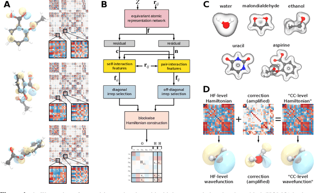
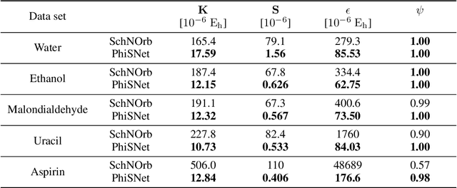
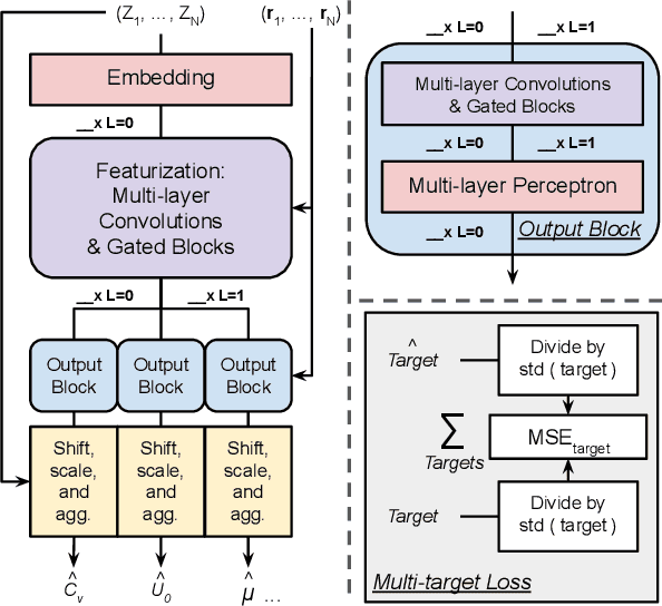
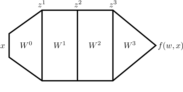
Machine learning has enabled the prediction of quantum chemical properties with high accuracy and efficiency, allowing to bypass computationally costly ab initio calculations. Instead of training on a fixed set of properties, more recent approaches attempt to learn the electronic wavefunction (or density) as a central quantity of atomistic systems, from which all other observables can be derived. This is complicated by the fact that wavefunctions transform non-trivially under molecular rotations, which makes them a challenging prediction target. To solve this issue, we introduce general SE(3)-equivariant operations and building blocks for constructing deep learning architectures for geometric point cloud data and apply them to reconstruct wavefunctions of atomistic systems with unprecedented accuracy. Our model reduces prediction errors by up to two orders of magnitude compared to the previous state-of-the-art and makes it possible to derive properties such as energies and forces directly from the wavefunction in an end-to-end manner. We demonstrate the potential of our approach in a transfer learning application, where a model trained on low accuracy reference wavefunctions implicitly learns to correct for electronic many-body interactions from observables computed at a higher level of theory. Such machine-learned wavefunction surrogates pave the way towards novel semi-empirical methods, offering resolution at an electronic level while drastically decreasing computational cost. While we focus on physics applications in this contribution, the proposed equivariant framework for deep learning on point clouds is promising also beyond, say, in computer vision or graphics.

Relative stability toward diffeomorphisms in deep nets indicates performance

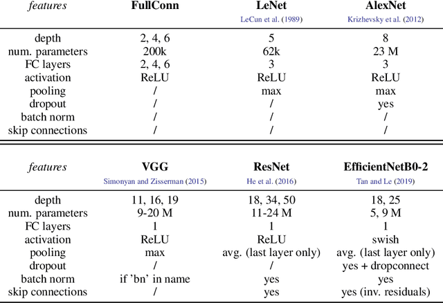
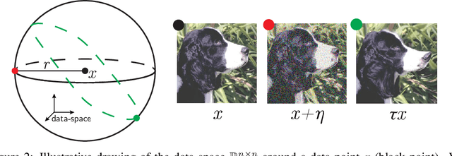
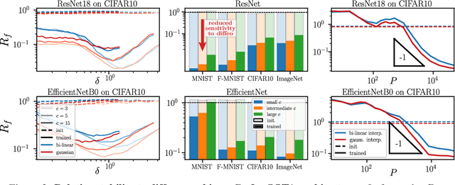
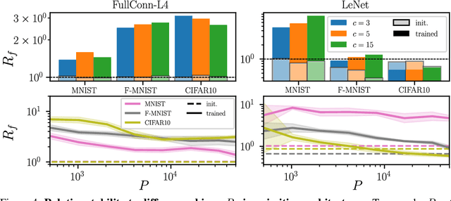
Understanding why deep nets can classify data in large dimensions remains a challenge. It has been proposed that they do so by becoming stable to diffeomorphisms, yet existing empirical measurements support that it is often not the case. We revisit this question by defining a maximum-entropy distribution on diffeomorphisms, that allows to study typical diffeomorphisms of a given norm. We confirm that stability toward diffeomorphisms does not strongly correlate to performance on four benchmark data sets of images. By contrast, we find that the stability toward diffeomorphisms relative to that of generic transformations $R_f$ correlates remarkably with the test error $\epsilon_t$. It is of order unity at initialization but decreases by several decades during training for state-of-the-art architectures. For CIFAR10 and 15 known architectures, we find $\epsilon_t\approx 0.2\sqrt{R_f}$, suggesting that obtaining a small $R_f$ is important to achieve good performance. We study how $R_f$ depends on the size of the training set and compare it to a simple model of invariant learning.

Perspective: A Phase Diagram for Deep Learning unifying Jamming, Feature Learning and Lazy Training

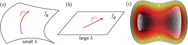
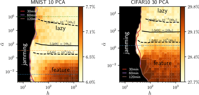
Deep learning algorithms are responsible for a technological revolution in a variety of tasks including image recognition or Go playing. Yet, why they work is not understood. Ultimately, they manage to classify data lying in high dimension -- a feat generically impossible due to the geometry of high dimensional space and the associated curse of dimensionality. Understanding what kind of structure, symmetry or invariance makes data such as images learnable is a fundamental challenge. Other puzzles include that (i) learning corresponds to minimizing a loss in high dimension, which is in general not convex and could well get stuck bad minima. (ii) Deep learning predicting power increases with the number of fitting parameters, even in a regime where data are perfectly fitted. In this manuscript, we review recent results elucidating (i,ii) and the perspective they offer on the (still unexplained) curse of dimensionality paradox. We base our theoretical discussion on the $(h,\alpha)$ plane where $h$ is the network width and $\alpha$ the scale of the output of the network at initialization, and provide new systematic measures of performance in that plane for MNIST and CIFAR 10. We argue that different learning regimes can be organized into a phase diagram. A line of critical points sharply delimits an under-parametrised phase from an over-parametrized one. In over-parametrized nets, learning can operate in two regimes separated by a smooth cross-over. At large initialization, it corresponds to a kernel method, whereas for small initializations features can be learnt, together with invariants in the data. We review the properties of these different phases, of the transition separating them and some open questions. Our treatment emphasizes analogies with physical systems, scaling arguments and the development of numerical observables to quantitatively test these results empirically.

Geometric compression of invariant manifolds in neural nets

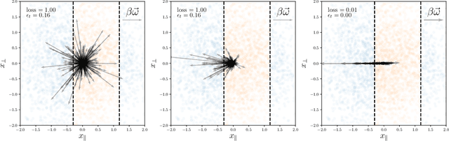
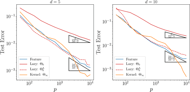
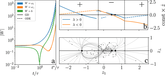
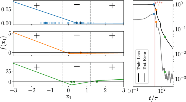
We study how neural networks compress uninformative input space in models where data lie in $d$ dimensions, but whose label only vary within a linear manifold of dimension $d_\parallel < d$. We show that for a one-hidden layer network initialized with infinitesimal weights (i.e. in the \textit{feature learning} regime) trained with gradient descent, the uninformative $d_\perp=d-d_\parallel$ space is compressed by a factor $\lambda\sim \sqrt{p}$, where $p$ is the size of the training set. We quantify the benefit of such a compression on the test error $\epsilon$. For large initialization of the weights (the \textit{lazy training} regime), no compression occurs and for regular boundaries separating labels we find that $\epsilon \sim p^{-\beta}$, with $\beta_\text{Lazy} = d / (3d-2)$. Compression improves the learning curves so that $\beta_\text{Feature} = (2d-1)/(3d-2)$ if $d_\parallel = 1$ and $\beta_\text{Feature} = (d + d_\perp/2)/(3d-2)$ if $d_\parallel > 1$. We test these predictions for a stripe model where boundaries are parallel interfaces ($d_\parallel=1$) as well as for a cylindrical boundary ($d_\parallel=2$). Next we show that compression shapes the Neural Tangent Kernel (NTK) evolution in time, so that its top eigenvectors become more informative and display a larger projection on the labels. Consequently, kernel learning with the frozen NTK at the end of training outperforms the initial NTK. We confirm these predictions both for a one-hidden layer FC network trained on the stripe model and for a 16-layers CNN trained on MNIST, for which we also find $\beta_\text{Feature}>\beta_\text{Lazy}$. The great similarities found in these two cases support that compression is central to the training of MNIST, and puts forward kernel-PCA on the evolving NTK as a useful diagnostic of compression in deep nets.

Relevance of Rotationally Equivariant Convolutions for Predicting Molecular Properties

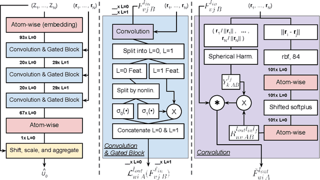
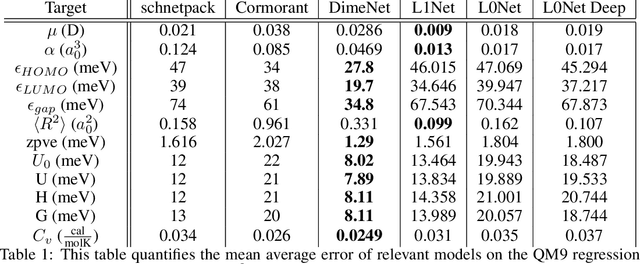
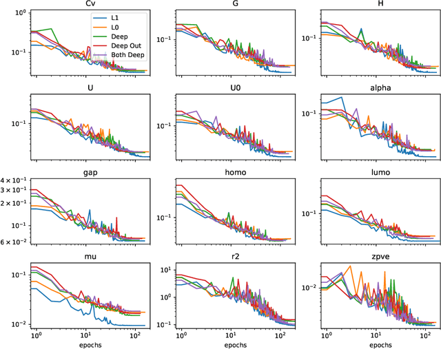
Equivariant neural networks (ENNs) are graph neural networks embedded in $\mathbb{R}^3$ and are well suited for predicting molecular properties. The ENN library e3nn has customizable convolutions, which can be designed to depend only on distances between points, or also on angular features, making them rotationally invariant, or equivariant, respectively. This paper studies the practical value of including angular dependencies for molecular property prediction using the QM9 data set. We find that for fixed network depth, adding angular features improves the accuracy on most targets. For most, but not all, molecular properties, distance-only e3nns (L0Nets) can compensate by increasing convolutional layer depth. Our angular-feature e3nn (L1Net) architecture beats previous state-of-the-art results on the global electronic properties dipole moment, isotropic polarizability, and electronic spatial extent.

Finding Symmetry Breaking Order Parameters with Euclidean Neural Networks

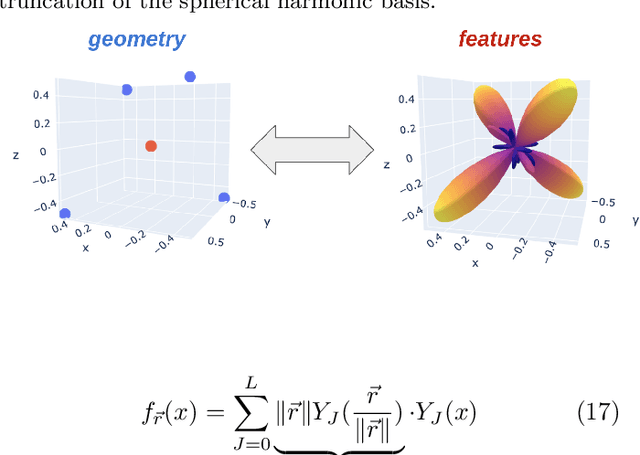
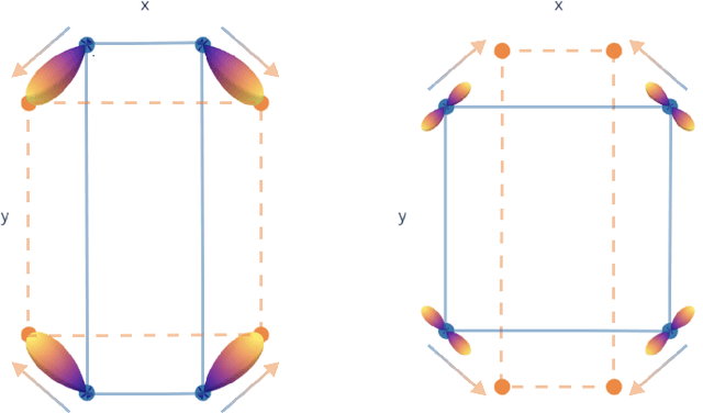
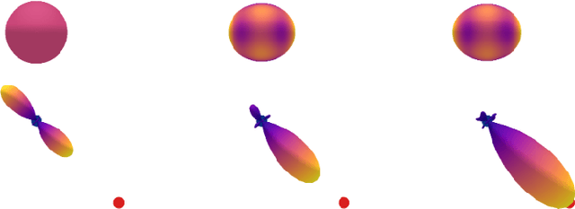
Curie's principle states that "when effects show certain asymmetry, this asymmetry must be found in the causes that gave rise to them". We demonstrate that symmetry equivariant neural networks uphold Curie's principle and this property can be used to uncover symmetry breaking order parameters necessary to make input and output data symmetrically compatible. We prove these properties mathematically and demonstrate them numerically by training a Euclidean symmetry equivariant neural network to learn symmetry breaking input to deform a square into a rectangle.

Disentangling feature and lazy learning in deep neural networks: an empirical study

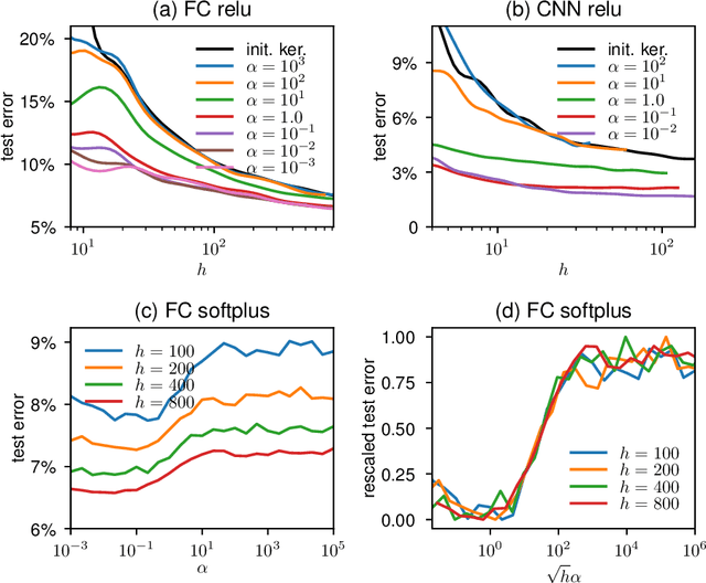
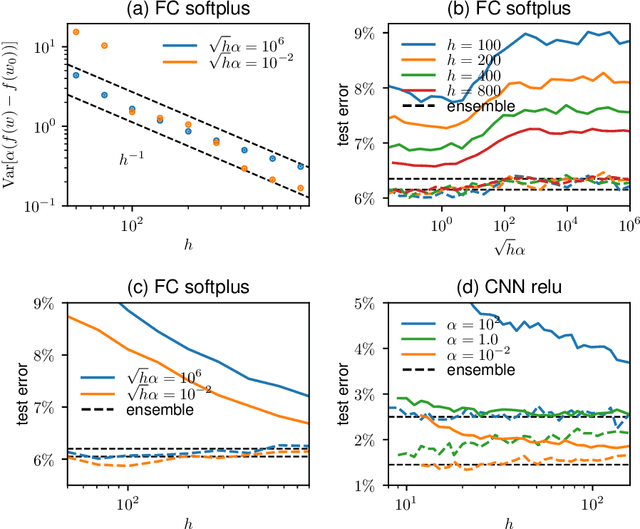
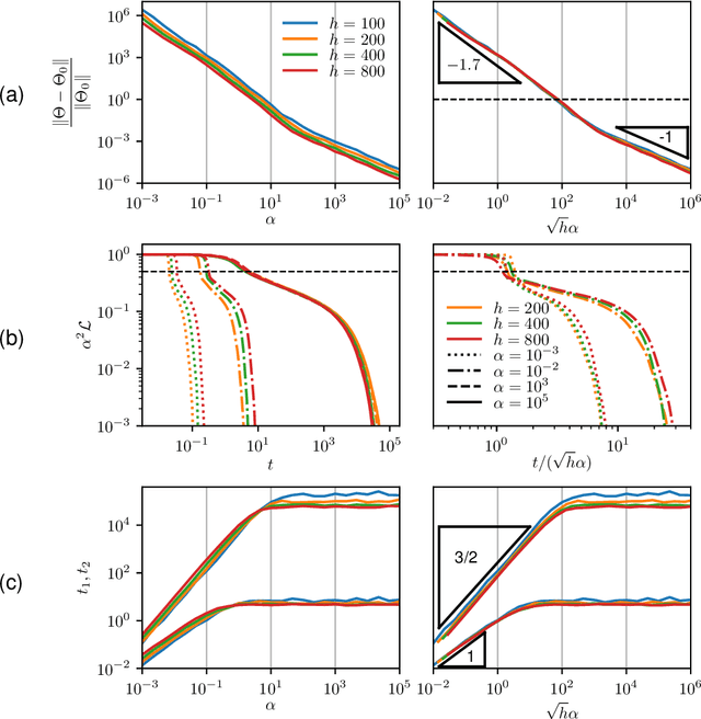
Two distinct limits for deep learning as the net width $h\to\infty$ have been proposed, depending on how the weights of the last layer scale with $h$. In the "lazy-learning" regime, the dynamics becomes linear in the weights and is described by a Neural Tangent Kernel $\Theta$. By contrast, in the "feature-learning" regime, the dynamics can be expressed in terms of the density distribution of the weights. Understanding which regime describes accurately practical architectures and which one leads to better performance remains a challenge. We answer these questions and produce new characterizations of these regimes for the MNIST data set, by considering deep nets $f$ whose last layer of weights scales as $\frac{\alpha}{\sqrt{h}}$ at initialization, where $\alpha$ is a parameter we vary. We performed systematic experiments on two setups (A) fully-connected Softplus momentum full batch and (B) convolutional ReLU momentum stochastic. We find that (1) $\alpha^*=\frac{1}{\sqrt{h}}$ separates the two regimes. (2) for (A) and (B) feature learning outperforms lazy learning, a difference in performance that decreases with $h$ and becomes hardly detectable asymptotically for (A) but is very significant for (B). (3) In both regimes, the fluctuations $\delta f$ induced by initial conditions on the learned function follow $\delta f\sim1/\sqrt{h}$, leading to a performance that increases with $h$. This improvement can be instead obtained at intermediate $h$ values by ensemble averaging different networks. (4) In the feature regime there exists a time scale $t_1\sim\alpha\sqrt{h}$, such that for $t\ll t_1$ the dynamics is linear. At $t\sim t_1$, the output has grown by a magnitude $\sqrt{h}$ and the changes of the tangent kernel $\|\Delta\Theta\|$ become significant. Ultimately, it follows $\|\Delta\Theta\|\sim(\sqrt{h}\alpha)^{-a}$ for ReLU and Softplus activation, with $a<2$ & $a\to2$ when depth grows.

Asymptotic learning curves of kernel methods: empirical data v.s. Teacher-Student paradigm

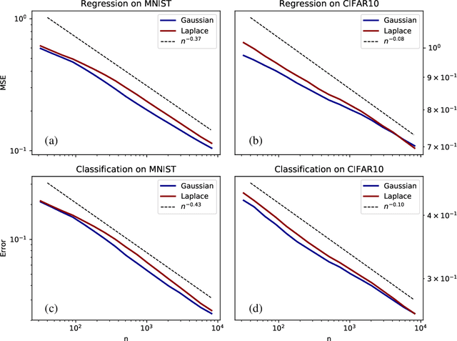
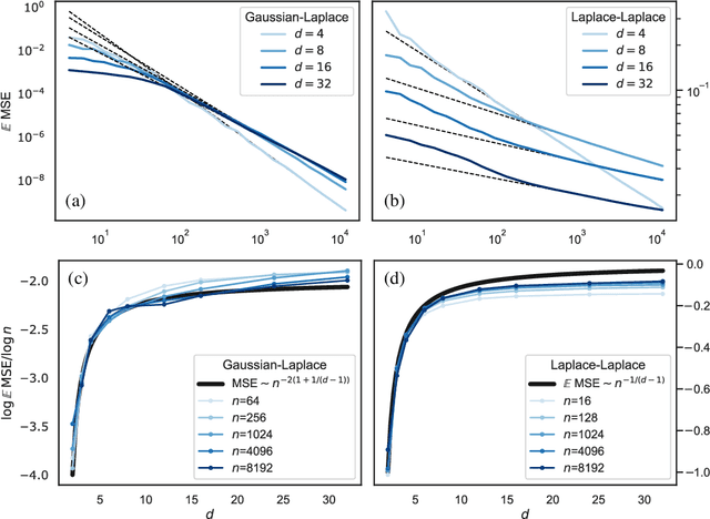
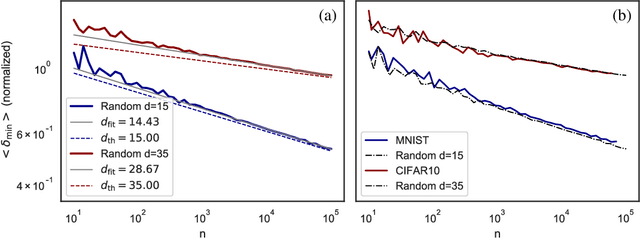
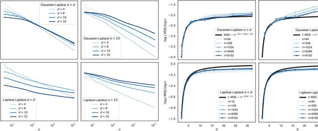
How many training data are needed to learn a supervised task? It is often observed that the generalization error decreases as $n^{-\beta}$ where $n$ is the number of training examples and $\beta$ an exponent that depends on both data and algorithm. In this work we measure $\beta$ when applying kernel methods to real datasets. For MNIST we find $\beta\approx 0.4$ and for CIFAR10 $\beta\approx 0.1$. Remarkably, $\beta$ is the same for regression and classification tasks, and for Gaussian or Laplace kernels. To rationalize the existence of non-trivial exponents that can be independent of the specific kernel used, we introduce the Teacher-Student framework for kernels. In this scheme, a Teacher generates data according to a Gaussian random field, and a Student learns them via kernel regression. With a simplifying assumption --- namely that the data are sampled from a regular lattice --- we derive analytically $\beta$ for translation invariant kernels, using previous results from the kriging literature. Provided that the Student is not too sensitive to high frequencies, $\beta$ depends only on the training data and their dimension. We confirm numerically that these predictions hold when the training points are sampled at random on a hypersphere. Overall, our results quantify how smooth Gaussian data should be to avoid the curse of dimensionality, and indicate that for kernel learning the relevant dimension of the data should be defined in terms of how the distance between nearest data points depends on $n$. With this definition one obtains reasonable effective smoothness estimates for MNIST and CIFAR10.

Scaling description of generalization with number of parameters in deep learning

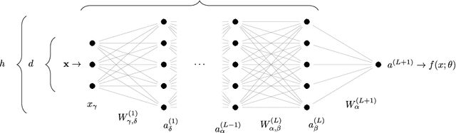
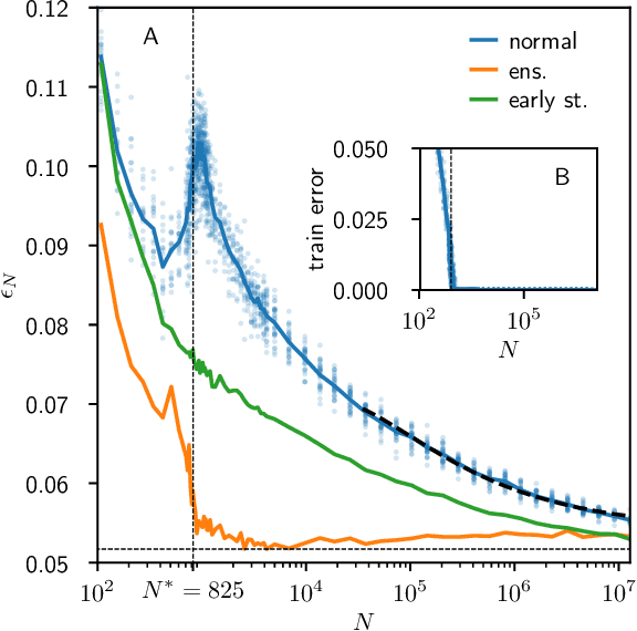
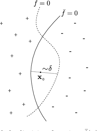
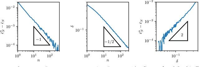
We provide a description for the evolution of the generalization performance of fixed-depth fully-connected deep neural networks as a function of the number of parameters $N$. We observe that increasing $N$ at fixed depth reduces the fluctuations of the output function $f_N$ induced by initial conditions, with $\Vert f_N-{\bar f}_N\Vert\sim N^{-1/4}$ where ${\bar f}_N$ denotes an average over initial conditions, and we explain this asymptotic behavior in terms of the fluctuations of the so-called Neural Tangent Kernel that controls the dynamics of the output function. For the task of classification, we predict these fluctuations to increase the test error $\epsilon$ as $\epsilon_{N}-\epsilon_{\infty}\sim N^{-1/2} + \mathcal{O}( N^{-3/4})$: this prediction is consistent with our empirical results on the MNIST dataset and it explains the puzzling observation that the predictive power of deep networks improves as the number of fitting parameters grows. This asymptotic description breaks down at a so-called jamming transition which takes place at a critical $N=N^*$, below which the training error is non-zero. In the absence of regularization, we observe an apparent divergence $\Vert f_N\Vert\sim (N-N^*)^{-\alpha}$ and provide a simple argument suggesting $\alpha=1$, consistent with empirical observations. This result leads to a plausible explanation for the cusp in test error known to occur at $N^*$. In practice, our analysis suggests that optimal generalization can be reached by ensemble averaging output functions at $N$ fixed slightly above $N^*$.

A General Theory of Equivariant CNNs on Homogeneous Spaces

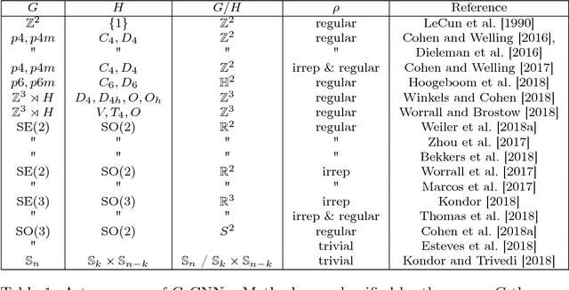
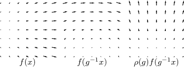
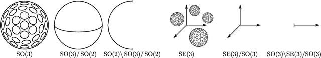
Group equivariant convolutional neural networks (G-CNNs) have recently emerged as a very effective model class for learning from signals in the context of known symmetries. A wide variety of equivariant layers has been proposed for signals on 2D and 3D Euclidean space, graphs, and the sphere, and it has become difficult to see how all of these methods are related, and how they may be generalized. In this paper, we present a fairly general theory of equivariant convolutional networks. Convolutional feature spaces are described as fields over a homogeneous base space, such as the plane $\mathbb{R}^2$, sphere $S^2$ or a graph $\mathcal{G}$. The theory enables a systematic classification of all existing G-CNNs in terms of their group of symmetry, base space, and field type (e.g. scalar, vector, or tensor field, etc.). In addition to this classification, we use Mackey theory to show that convolutions with equivariant kernels are the most general class of equivariant maps between such fields, thus establishing G-CNNs as a universal class of equivariant networks. The theory also explains how the space of equivariant kernels can be parameterized for learning, thereby simplifying the development of G-CNNs for new spaces and symmetries. Finally, the theory introduces a rich geometric semantics to learned feature spaces, thus improving interpretability of deep networks, and establishing a connection to central ideas in mathematics and physics.