Score-based diffusion nowcasting of GOES imagery

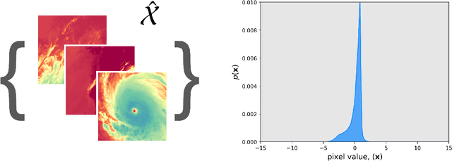
Clouds and precipitation are important for understanding weather and climate. Simulating clouds and precipitation with traditional numerical weather prediction is challenging because of the sub-grid parameterizations required. Machine learning has been explored for forecasting clouds and precipitation, but early machine learning methods often created blurry forecasts. In this paper we explore a newer method, named score-based diffusion, to nowcast (zero to three hour forecast) clouds and precipitation. We discuss the background and intuition of score-based diffusion models - thus providing a starting point for the community - while exploring the methodology's use for nowcasting geostationary infrared imagery. We experiment with three main types of diffusion models: a standard score-based diffusion model (Diff); a residual correction diffusion model (CorrDiff); and a latent diffusion model (LDM). Our results show that the diffusion models are able to not only advect existing clouds, but also generate and decay clouds, including convective initiation. These results are surprising because the forecasts are initiated with only the past 20 mins of infrared satellite imagery. A case study qualitatively shows the preservation of high resolution features longer into the forecast than a conventional mean-squared error trained U-Net. The best of the three diffusion models tested was the CorrDiff approach, outperforming all other diffusion models, the traditional U-Net, and a persistence forecast by one to two kelvin on root mean squared error. The diffusion models also enable out-of-the-box ensemble generation, which shows skillful calibration, with the spread of the ensemble correlating well to the error.

Center-fixing of tropical cyclones using uncertainty-aware deep learning applied to high-temporal-resolution geostationary satellite imagery

Determining the location of a tropical cyclone's (TC) surface circulation center -- "center-fixing" -- is a critical first step in the TC-forecasting process, affecting current and future estimates of track, intensity, and structure. Despite a recent increase in the number of automated center-fixing methods, only one such method (ARCHER-2) is operational, and its best performance is achieved when using microwave or scatterometer data, which are not available at every forecast cycle. We develop a deep-learning algorithm called GeoCenter; it relies only on geostationary IR satellite imagery, which is available for all TC basins at high frequency (10-15 min) and low latency (< 10 min) during both day and night. GeoCenter ingests an animation (time series) of IR images, including 10 channels at lag times up to 3 hours. The animation is centered at a "first guess" location, offset from the true TC-center location by 48 km on average and sometimes > 100 km; GeoCenter is tasked with correcting this offset. On an independent testing dataset, GeoCenter achieves a mean/median/RMS (root mean square) error of 26.9/23.3/32.0 km for all systems, 25.7/22.3/30.5 km for tropical systems, and 15.7/13.6/18.6 km for category-2--5 hurricanes. These values are similar to ARCHER-2 errors when microwave or scatterometer data are available, and better than ARCHER-2 errors when only IR data are available. GeoCenter also performs skillful uncertainty quantification (UQ), producing a well calibrated ensemble of 200 TC-center locations. Furthermore, all predictors used by GeoCenter are available in real time, which would make GeoCenter easy to implement operationally every 10-15 min.

Evaluation of Tropical Cyclone Track and Intensity Forecasts from Artificial Intelligence Weather Prediction (AIWP) Models

In just the past few years multiple data-driven Artificial Intelligence Weather Prediction (AIWP) models have been developed, with new versions appearing almost monthly. Given this rapid development, the applicability of these models to operational forecasting has yet to be adequately explored and documented. To assess their utility for operational tropical cyclone (TC) forecasting, the NHC verification procedure is used to evaluate seven-day track and intensity predictions for northern hemisphere TCs from May-November 2023. Four open-source AIWP models are considered (FourCastNetv1, FourCastNetv2-small, GraphCast-operational and Pangu-Weather). The AIWP track forecast errors and detection rates are comparable to those from the best-performing operational forecast models. However, the AIWP intensity forecast errors are larger than those of even the simplest intensity forecasts based on climatology and persistence. The AIWP models almost always reduce the TC intensity, especially within the first 24 h of the forecast, resulting in a substantial low bias. The contribution of the AIWP models to the NHC model consensus was also evaluated. The consensus track errors are reduced by up to 11% at the longer time periods. The five-day NHC official track forecasts have improved by about 2% per year since 2001, so this represents more than a five-year gain in accuracy. Despite substantial negative intensity biases, the AIWP models have a neutral impact on the intensity consensus. These results show that the current formulation of the AIWP models have promise for operational TC track forecasts, but improved bias corrections or model reformulations will be needed for accurate intensity forecasts.

SRViT: Vision Transformers for Estimating Radar Reflectivity from Satellite Observations at Scale

We introduce a transformer-based neural network to generate high-resolution (3km) synthetic radar reflectivity fields at scale from geostationary satellite imagery. This work aims to enhance short-term convective-scale forecasts of high-impact weather events and aid in data assimilation for numerical weather prediction over the United States. Compared to convolutional approaches, which have limited receptive fields, our results show improved sharpness and higher accuracy across various composite reflectivity thresholds. Additional case studies over specific atmospheric phenomena support our quantitative findings, while a novel attribution method is introduced to guide domain experts in understanding model outputs.

Carefully choose the baseline: Lessons learned from applying XAI attribution methods for regression tasks in geoscience

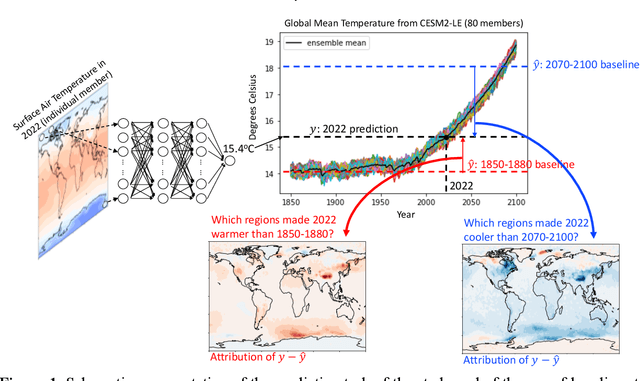
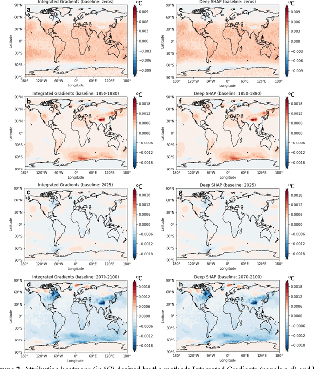
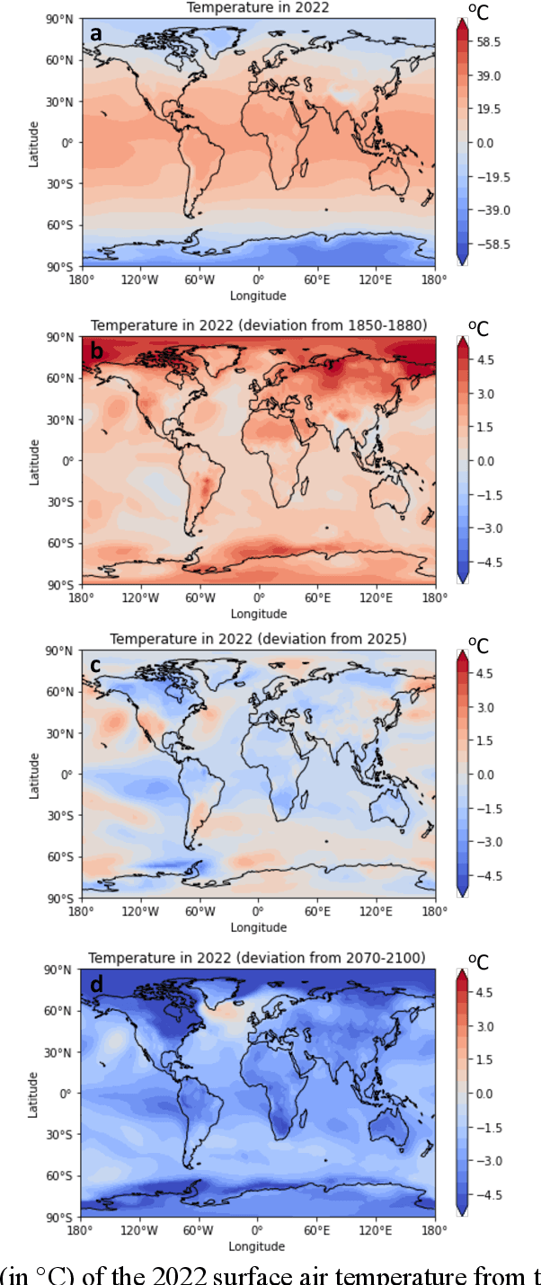
Methods of eXplainable Artificial Intelligence (XAI) are used in geoscientific applications to gain insights into the decision-making strategy of Neural Networks (NNs) highlighting which features in the input contribute the most to a NN prediction. Here, we discuss our lesson learned that the task of attributing a prediction to the input does not have a single solution. Instead, the attribution results and their interpretation depend greatly on the considered baseline (sometimes referred to as reference point) that the XAI method utilizes; a fact that has been overlooked so far in the literature. This baseline can be chosen by the user or it is set by construction in the method s algorithm, often without the user being aware of that choice. We highlight that different baselines can lead to different insights for different science questions and, thus, should be chosen accordingly. To illustrate the impact of the baseline, we use a large ensemble of historical and future climate simulations forced with the SSP3-7.0 scenario and train a fully connected NN to predict the ensemble- and global-mean temperature (i.e., the forced global warming signal) given an annual temperature map from an individual ensemble member. We then use various XAI methods and different baselines to attribute the network predictions to the input. We show that attributions differ substantially when considering different baselines, as they correspond to answering different science questions. We conclude by discussing some important implications and considerations about the use of baselines in XAI research.

A Primer on Topological Data Analysis to Support Image Analysis Tasks in Environmental Science

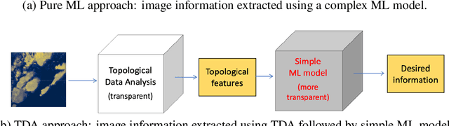
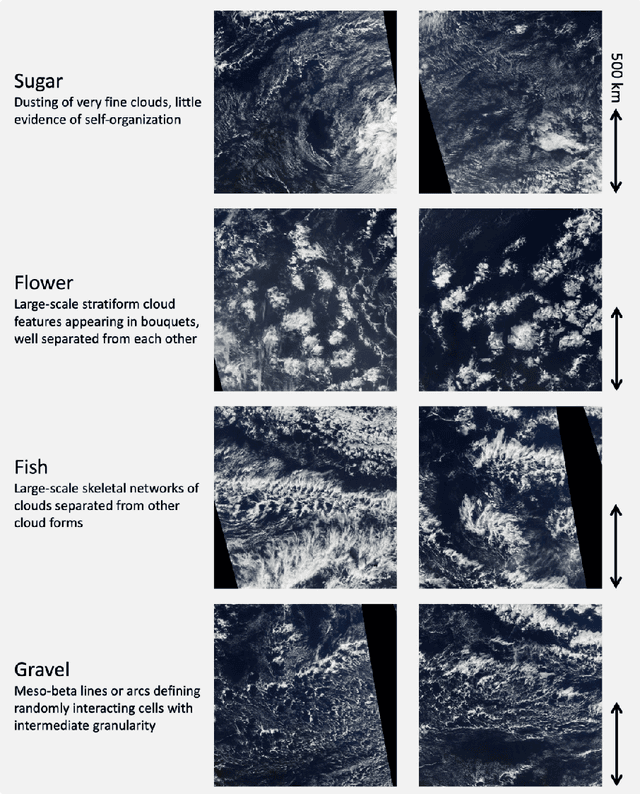
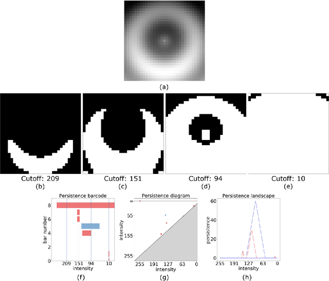
Topological data analysis (TDA) is a tool from data science and mathematics that is beginning to make waves in environmental science. In this work, we seek to provide an intuitive and understandable introduction to a tool from TDA that is particularly useful for the analysis of imagery, namely persistent homology. We briefly discuss the theoretical background but focus primarily on understanding the output of this tool and discussing what information it can glean. To this end, we frame our discussion around a guiding example of classifying satellite images from the Sugar, Fish, Flower, and Gravel Dataset produced for the study of mesocale organization of clouds by Rasp et. al. in 2020 (arXiv:1906:01906). We demonstrate how persistent homology and its vectorization, persistence landscapes, can be used in a workflow with a simple machine learning algorithm to obtain good results, and explore in detail how we can explain this behavior in terms of image-level features. One of the core strengths of persistent homology is how interpretable it can be, so throughout this paper we discuss not just the patterns we find, but why those results are to be expected given what we know about the theory of persistent homology. Our goal is that a reader of this paper will leave with a better understanding of TDA and persistent homology, be able to identify problems and datasets of their own for which persistent homology could be helpful, and gain an understanding of results they obtain from applying the included GitHub example code.

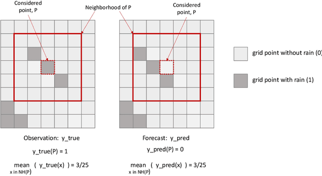
Can we integrate spatial verification methods into neural-network loss functions for atmospheric science?

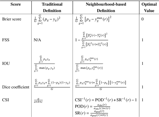
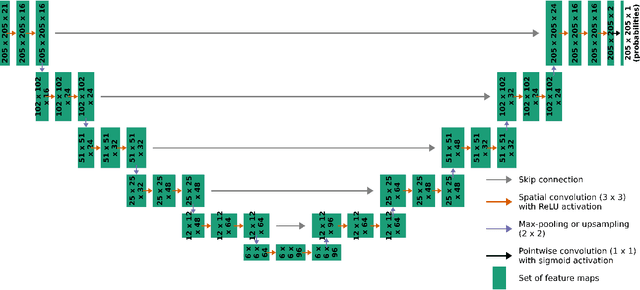
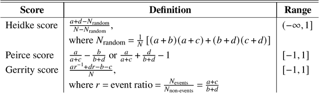
In the last decade, much work in atmospheric science has focused on spatial verification (SV) methods for gridded prediction, which overcome serious disadvantages of pixelwise verification. However, neural networks (NN) in atmospheric science are almost always trained to optimize pixelwise loss functions, even when ultimately assessed with SV methods. This establishes a disconnect between model verification during vs. after training. To address this issue, we develop spatially enhanced loss functions (SELF) and demonstrate their use for a real-world problem: predicting the occurrence of thunderstorms (henceforth, "convection") with NNs. In each SELF we use either a neighbourhood filter, which highlights convection at scales larger than a threshold, or a spectral filter (employing Fourier or wavelet decomposition), which is more flexible and highlights convection at scales between two thresholds. We use these filters to spatially enhance common verification scores, such as the Brier score. We train each NN with a different SELF and compare their performance at many scales of convection, from discrete storm cells to tropical cyclones. Among our many findings are that (a) for a low (high) risk threshold, the ideal SELF focuses on small (large) scales; (b) models trained with a pixelwise loss function perform surprisingly well; (c) however, models trained with a spectral filter produce better-calibrated probabilities than a pixelwise model. We provide a general guide to using SELFs, including technical challenges and the final Python code, as well as demonstrating their use for the convection problem. To our knowledge this is the most in-depth guide to SELFs in the geosciences.

Investigating the fidelity of explainable artificial intelligence methods for applications of convolutional neural networks in geoscience

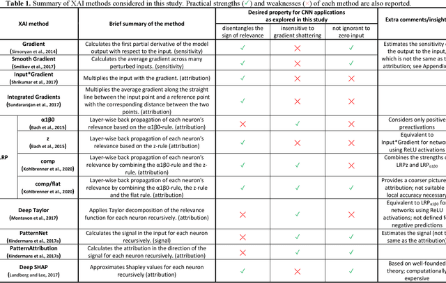
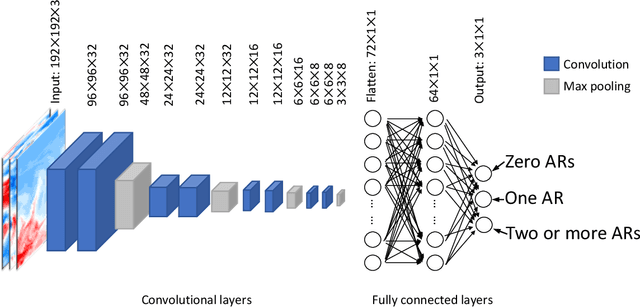
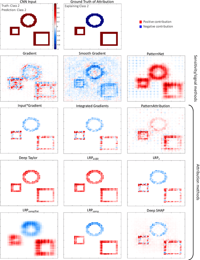
Convolutional neural networks (CNNs) have recently attracted great attention in geoscience due to their ability to capture non-linear system behavior and extract predictive spatiotemporal patterns. Given their black-box nature however, and the importance of prediction explainability, methods of explainable artificial intelligence (XAI) are gaining popularity as a means to explain the CNN decision-making strategy. Here, we establish an intercomparison of some of the most popular XAI methods and investigate their fidelity in explaining CNN decisions for geoscientific applications. Our goal is to raise awareness of the theoretical limitations of these methods and gain insight into the relative strengths and weaknesses to help guide best practices. The considered XAI methods are first applied to an idealized attribution benchmark, where the ground truth of explanation of the network is known a priori, to help objectively assess their performance. Secondly, we apply XAI to a climate-related prediction setting, namely to explain a CNN that is trained to predict the number of atmospheric rivers in daily snapshots of climate simulations. Our results highlight several important issues of XAI methods (e.g., gradient shattering, inability to distinguish the sign of attribution, ignorance to zero input) that have previously been overlooked in our field and, if not considered cautiously, may lead to a distorted picture of the CNN decision-making strategy. We envision that our analysis will motivate further investigation into XAI fidelity and will help towards a cautious implementation of XAI in geoscience, which can lead to further exploitation of CNNs and deep learning for prediction problems.

The Need for Ethical, Responsible, and Trustworthy Artificial Intelligence for Environmental Sciences

Given the growing use of Artificial Intelligence (AI) and machine learning (ML) methods across all aspects of environmental sciences, it is imperative that we initiate a discussion about the ethical and responsible use of AI. In fact, much can be learned from other domains where AI was introduced, often with the best of intentions, yet often led to unintended societal consequences, such as hard coding racial bias in the criminal justice system or increasing economic inequality through the financial system. A common misconception is that the environmental sciences are immune to such unintended consequences when AI is being used, as most data come from observations, and AI algorithms are based on mathematical formulas, which are often seen as objective. In this article, we argue the opposite can be the case. Using specific examples, we demonstrate many ways in which the use of AI can introduce similar consequences in the environmental sciences. This article will stimulate discussion and research efforts in this direction. As a community, we should avoid repeating any foreseeable mistakes made in other domains through the introduction of AI. In fact, with proper precautions, AI can be a great tool to help {\it reduce} climate and environmental injustice. We primarily focus on weather and climate examples but the conclusions apply broadly across the environmental sciences.

CIRA Guide to Custom Loss Functions for Neural Networks in Environmental Sciences -- Version 1

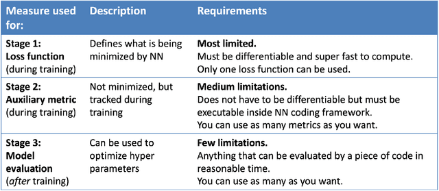
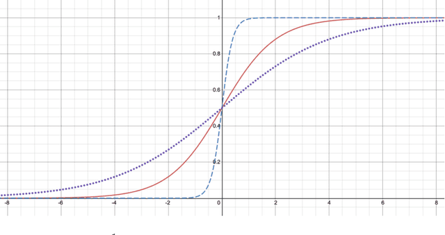
Neural networks are increasingly used in environmental science applications. Furthermore, neural network models are trained by minimizing a loss function, and it is crucial to choose the loss function very carefully for environmental science applications, as it determines what exactly is being optimized. Standard loss functions do not cover all the needs of the environmental sciences, which makes it important for scientists to be able to develop their own custom loss functions so that they can implement many of the classic performance measures already developed in environmental science, including measures developed for spatial model verification. However, there are very few resources available that cover the basics of custom loss function development comprehensively, and to the best of our knowledge none that focus on the needs of environmental scientists. This document seeks to fill this gap by providing a guide on how to write custom loss functions targeted toward environmental science applications. Topics include the basics of writing custom loss functions, common pitfalls, functions to use in loss functions, examples such as fractions skill score as loss function, how to incorporate physical constraints, discrete and soft discretization, and concepts such as focal, robust, and adaptive loss. While examples are currently provided in this guide for Python with Keras and the TensorFlow backend, the basic concepts also apply to other environments, such as Python with PyTorch. Similarly, while the sample loss functions provided here are from meteorology, these are just examples of how to create custom loss functions. Other fields in the environmental sciences have very similar needs for custom loss functions, e.g., for evaluating spatial forecasts effectively, and the concepts discussed here can be applied there as well. All code samples are provided in a GitHub repository.