Circuit design in biology and machine learning. I. Random networks and dimensional reduction

A biological circuit is a neural or biochemical cascade, taking inputs and producing outputs. How have biological circuits learned to solve environmental challenges over the history of life? The answer certainly follows Dobzhansky's famous quote that ``nothing in biology makes sense except in the light of evolution.'' But that quote leaves out the mechanistic basis by which natural selection's trial-and-error learning happens, which is exactly what we have to understand. How does the learning process that designs biological circuits actually work? How much insight can we gain about the form and function of biological circuits by studying the processes that have made those circuits? Because life's circuits must often solve the same problems as those faced by machine learning, such as environmental tracking, homeostatic control, dimensional reduction, or classification, we can begin by considering how machine learning designs computational circuits to solve problems. We can then ask: How much insight do those computational circuits provide about the design of biological circuits? How much does biology differ from computers in the particular circuit designs that it uses to solve problems? This article steps through two classic machine learning models to set the foundation for analyzing broad questions about the design of biological circuits. One insight is the surprising power of randomly connected networks. Another is the central role of internal models of the environment embedded within biological circuits, illustrated by a model of dimensional reduction and trend prediction. Overall, many challenges in biology have machine learning analogs, suggesting hypotheses about how biology's circuits are designed.

Automatic differentiation and the optimization of differential equation models in biology

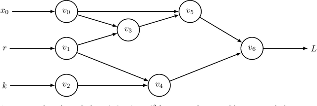
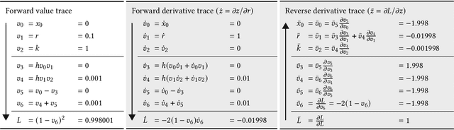
A computational revolution unleashed the power of artificial neural networks. At the heart of that revolution is automatic differentiation, which calculates the derivative of a performance measure relative to a large number of parameters. Differentiation enhances the discovery of improved performance in large models, an achievement that was previously difficult or impossible. Recently, a second computational advance optimizes the temporal trajectories traced by differential equations. Optimization requires differentiating a measure of performance over a trajectory, such as the closeness of tracking the environment, with respect to the parameters of the differential equations. Because model trajectories are usually calculated numerically by multistep algorithms, such as Runge-Kutta, the automatic differentiation must be passed through the numerical algorithm. This article explains how such automatic differentiation of trajectories is achieved. It also discusses why such computational breakthroughs are likely to advance theoretical and statistical studies of biological problems, in which one can consider variables as dynamic paths over time and space. Many common problems arise between improving success in computational learning models over performance landscapes, improving evolutionary fitness over adaptive landscapes, and improving statistical fits to data over information landscapes.

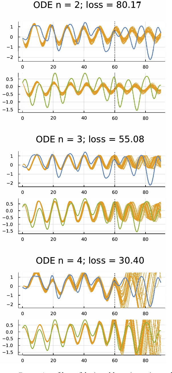
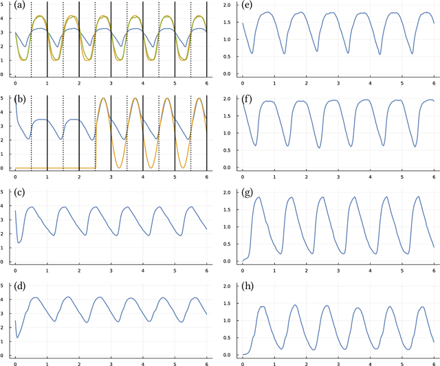
Optimizing differential equations to fit data and predict outcomes

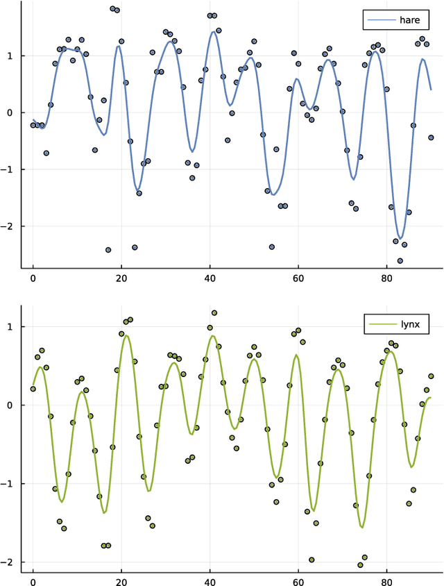
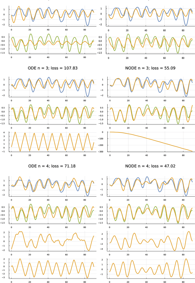
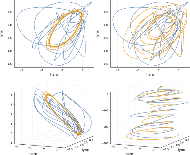
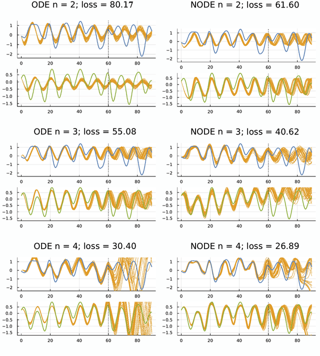
Many scientific problems focus on observed patterns of change or on how to design a system to achieve particular dynamics. Those problems often require fitting differential equation models to target trajectories. Fitting such models can be difficult because each evaluation of the fit must calculate the distance between the model and target patterns at numerous points along a trajectory. The gradient of the fit with respect to the model parameters can be challenging. Recent technical advances in automatic differentiation through numerical differential equation solvers potentially change the fitting process into a relatively easy problem, opening up new possibilities to study dynamics. However, application of the new tools to real data may fail to achieve a good fit. This article illustrates how to overcome a variety of common challenges, using the classic ecological data for oscillations in hare and lynx populations. Models include simple ordinary differential equations (ODEs) and neural ordinary differential equations (NODEs), which use artificial neural networks to estimate the derivatives of differential equation systems. Comparing the fits obtained with ODEs versus NODEs, representing small and large parameter spaces, and changing the number of variable dimensions provide insight into the geometry of the observed and model trajectories. To analyze the quality of the models for predicting future observations, a Bayesian-inspired preconditioned stochastic gradient Langevin dynamics (pSGLD) calculation of the posterior distribution of predicted model trajectories clarifies the tendency for various models to underfit or overfit the data. Coupling fitted differential equation systems with pSGLD sampling provides a powerful way to study the properties of optimization surfaces, raising an analogy with mutation-selection dynamics on fitness landscapes.

The inductive theory of natural selection: summary and synthesis

The theory of natural selection has two forms. Deductive theory describes how populations change over time. One starts with an initial population and some rules for change. From those assumptions, one calculates the future state of the population. Deductive theory predicts how populations adapt to environmental challenge. Inductive theory describes the causes of change in populations. One starts with a given amount of change. One then assigns different parts of the total change to particular causes. Inductive theory analyzes alternative causal models for how populations have adapted to environmental challenge. This chapter emphasizes the inductive analysis of cause.