Comment on "Machine learning conservation laws from differential equations"

In lieu of abstract, first paragraph reads: Six months after the author derived a constant of motion for a 1D damped harmonic oscillator [1], a similar result appeared by Liu, Madhavan, and Tegmark [2, 3], without citing the author. However, their derivation contained six serious errors, causing both their method and result to be incorrect. In this Comment, those errors are reviewed.

Constants of Motion for Conserved and Non-conserved Dynamics

This paper begins with a dynamical model that was obtained by applying a machine learning technique (FJet) to time-series data; this dynamical model is then analyzed with Lie symmetry techniques to obtain constants of motion. This analysis is performed on both the conserved and non-conserved cases of the 1D and 2D harmonic oscillators. For the 1D oscillator, constants are found in the cases where the system is underdamped, overdamped, and critically damped. The novel existence of such a constant for a non-conserved model is interpreted as a manifestation of the conservation of energy of the {\em total} system (i.e., oscillator plus dissipative environment). For the 2D oscillator, constants are found for the isotropic and anisotropic cases, including when the frequencies are incommensurate; it is also generalized to arbitrary dimensions. In addition, a constant is identified which generalizes angular momentum for all ratios of the frequencies. The approach presented here can produce {\em multiple} constants of motion from a {\em single}, generic data set.

Extracting Dynamical Models from Data

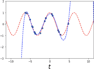
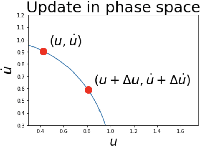
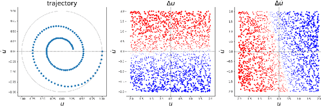
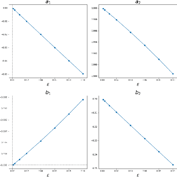
The FJet approach is introduced for determining the underlying model of data from a dynamical system. It borrows ideas from the fields of Lie symmetries as applied to differential equations (DEs), and numerical integration (such as Runge-Kutta). The technique can be considered as a way to use machine learning (ML) to derive a numerical integration scheme. The technique naturally overcomes the "extrapolation problem", which is when ML is used to extrapolate a model beyond the time range of the original training data. It does this by doing the modeling in the phase space of the system, rather than over the time domain. When modeled with a type of regression scheme, it's possible to accurately determine the underlying DE, along with parameter dependencies. Ideas from the field of Lie symmetries applied to ordinary DEs are used to determine constants of motion, even for damped and driven systems. These statements are demonstrated on three examples: a damped harmonic oscillator, a damped pendulum, and a damped, driven nonlinear oscillator (Duffing oscillator). In the model for the Duffing oscillator, it's possible to treat the external force in a manner reminiscent of a Green's function approach. Also, in the case of the undamped harmonic oscillator, the FJet approach remains stable approximately $10^9$ times longer than $4$th-order Runge-Kutta.

2nd-order Updates with 1st-order Complexity

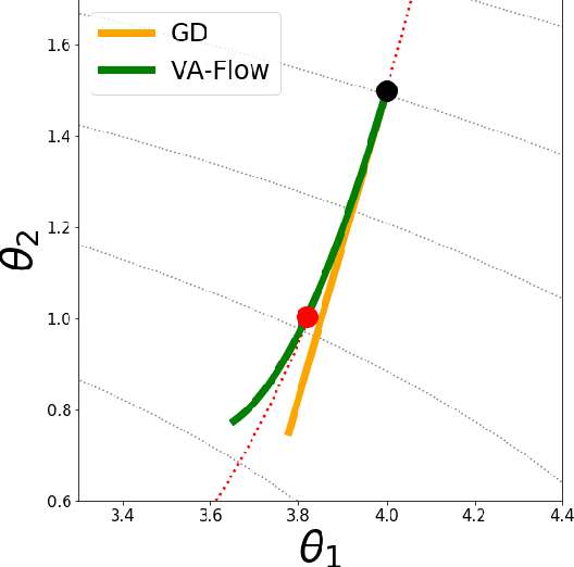
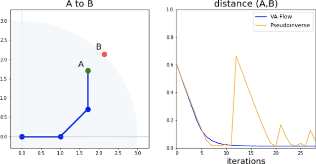
It has long been a goal to efficiently compute and use second order information on a function ($f$) to assist in numerical approximations. Here it is shown how, using only basic physics and a numerical approximation, such information can be accurately obtained at a cost of ${\cal O}(N)$ complexity, where $N$ is the dimensionality of the parameter space of $f$. In this paper, an algorithm ({\em VA-Flow}) is developed to exploit this second order information, and pseudocode is presented. It is applied to two classes of problems, that of inverse kinematics (IK) and gradient descent (GD). In the IK application, the algorithm is fast and robust, and is shown to lead to smooth behavior even near singularities. For GD the algorithm also works very well, provided the cost function is locally well-described by a polynomial.

Neograd: Gradient Descent with a Near-Ideal Learning Rate

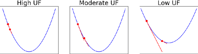
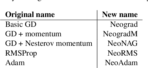
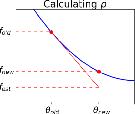
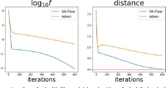
Since its inception by Cauchy in 1847, the gradient descent algorithm has been without guidance as to how to efficiently set the learning rate. This paper identifies a concept, defines metrics, and introduces algorithms to provide such guidance. The result is a family of algorithms (Neograd) based on a {\em constant $\rho$ ansatz}, where $\rho$ is a metric based on the error of the updates. This allows one to adjust the learning rate at each step, using a formulaic estimate based on $\rho$. It is now no longer necessary to do trial runs beforehand to estimate a single learning rate for an entire optimization run. The additional costs to operate this metric are trivial. One member of this family of algorithms, NeogradM, can quickly reach much lower cost function values than other first order algorithms. Comparisons are made mainly between NeogradM and Adam on an array of test functions and on a neural network model for identifying hand-written digits. The results show great performance improvements with NeogradM.

Speedup from a different parametrization within the Neural Network algorithm

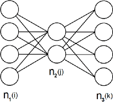
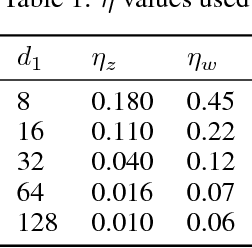
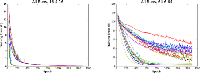
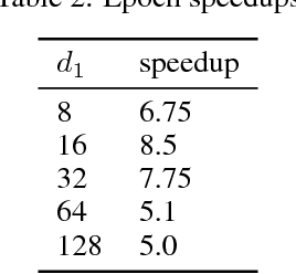
A different parametrization of the hyperplanes is used in the neural network algorithm. As demonstrated on several autoencoder examples it significantly outperforms the usual parametrization, reaching lower training error values with only a fraction of the number of epochs. It's argued that it makes it easier to understand and initialize the parameters.